import numpy as npnumpy공부 7단계
note 1: 메소드 도움말 확인하기
- 파이썬에서 함수를 적용하는 2가지 방식 - np.sum(a) - a.sum()
a=np.array([1,2,3,4,5])
a
array([1, 2, 3, 4, 5])a.sum()15np.sum(a)15- 넘파이에서 a.sum에 대한 도움말은 보통 np.sum()에 자세히 나와있음 \(\to\) np.sum()의 도움말을 확인하고 np.sum(a)와 a.sum()이 동일함을 이용하여 a.sum()의 사용법을 미루어 유추해야함
a.sum?np.sum?np.sum([0.5, 1.5])2.0note2: hstack, vstack
- hstack, vstack를 쓰는 사람도 있다.
a=np.arange(6)
b=-anp.vstack([a,b])array([[ 0, 1, 2, 3, 4, 5],
[ 0, -1, -2, -3, -4, -5]])np.stack([a,b],axis=0)array([[ 0, 1, 2, 3, 4, 5],
[ 0, -1, -2, -3, -4, -5]])np.hstack([a,b])array([ 0, 1, 2, 3, 4, 5, 0, -1, -2, -3, -4, -5])np.concatenate([a,b],axis=0)array([ 0, 1, 2, 3, 4, 5, 0, -1, -2, -3, -4, -5])note3: append
- 기능1:reshape(-1) + concat
a=np.arange(30).reshape(5,6)
b= -np.arange(8).reshape(2,2,2)
a.shape, b.shape((5, 6), (2, 2, 2))np.append(a,b)array([ 0, 1, 2, 3, 4, 5, 6, 7, 8, 9, 10, 11, 12, 13, 14, 15, 16,
17, 18, 19, 20, 21, 22, 23, 24, 25, 26, 27, 28, 29, 0, -1, -2, -3,
-4, -5, -6, -7])np.concatenate([a.reshape(-1), b.reshape(-1)])array([ 0, 1, 2, 3, 4, 5, 6, 7, 8, 9, 10, 11, 12, 13, 14, 15, 16,
17, 18, 19, 20, 21, 22, 23, 24, 25, 26, 27, 28, 29, 0, -1, -2, -3,
-4, -5, -6, -7])- 기능2: concat
a=np.arange(2*3*4).reshape(2,3,4)
b=-a
a.shape, b.shape, np.append(a,b, axis=0).shape # 대괄호를 쓰지 않아도 됨((2, 3, 4), (2, 3, 4), (4, 3, 4))a.shape, b.shape, np.append(a,b, axis=1).shape((2, 3, 4), (2, 3, 4), (2, 6, 4))a.shape, b.shape, np.append(a,b, axis=2).shape((2, 3, 4), (2, 3, 4), (2, 3, 8))- concat과의 차이?
a=np.arange(2*3*4).reshape(2,3,4)
b=-a
c=2*anp.concatenate([a,b,c],axis=0)array([[[ 0, 1, 2, 3],
[ 4, 5, 6, 7],
[ 8, 9, 10, 11]],
[[ 12, 13, 14, 15],
[ 16, 17, 18, 19],
[ 20, 21, 22, 23]],
[[ 0, -1, -2, -3],
[ -4, -5, -6, -7],
[ -8, -9, -10, -11]],
[[-12, -13, -14, -15],
[-16, -17, -18, -19],
[-20, -21, -22, -23]],
[[ 0, 2, 4, 6],
[ 8, 10, 12, 14],
[ 16, 18, 20, 22]],
[[ 24, 26, 28, 30],
[ 32, 34, 36, 38],
[ 40, 42, 44, 46]]])note4: revel, flatten
a=np.arange(2*3*4).reshape(2,3,4)
a
array([[[ 0, 1, 2, 3],
[ 4, 5, 6, 7],
[ 8, 9, 10, 11]],
[[12, 13, 14, 15],
[16, 17, 18, 19],
[20, 21, 22, 23]]])a.reshape(-1) #디멘전 1차원으로array([ 0, 1, 2, 3, 4, 5, 6, 7, 8, 9, 10, 11, 12, 13, 14, 15, 16,
17, 18, 19, 20, 21, 22, 23])a.ravel()array([ 0, 1, 2, 3, 4, 5, 6, 7, 8, 9, 10, 11, 12, 13, 14, 15, 16,
17, 18, 19, 20, 21, 22, 23])a.flatten()array([ 0, 1, 2, 3, 4, 5, 6, 7, 8, 9, 10, 11, 12, 13, 14, 15, 16,
17, 18, 19, 20, 21, 22, 23])note 5: 기타 통계함수들
- 평균, 중앙값, 표준편차, 분산
a=np.random.normal(loc=0, scale=2, size=(100,))
a
array([-2.01759369e+00, 1.70831942e+00, -7.66284153e-01, 2.15177363e+00,
1.93917905e+00, -2.74073590e-01, -2.04642372e+00, -1.98463689e+00,
1.83815582e+00, 4.49207271e+00, -5.40520993e-03, 1.45933943e+00,
-1.88730370e+00, 2.53422937e+00, -1.43846951e+00, -2.69938884e-01,
-2.68912083e+00, 6.01230062e-01, 1.21155692e+00, -1.78259314e+00,
3.08941967e-01, 1.22338707e+00, -1.03232597e+00, -1.79667669e+00,
2.19458228e+00, 5.75514508e-01, -3.02570319e+00, -1.21868604e+00,
-9.60932070e-01, 1.11771254e+00, -5.34063250e-01, -2.68962004e+00,
-4.62864312e+00, 4.64113175e+00, -1.05051461e+00, -6.14152261e-01,
-1.56320062e+00, 1.18863285e-01, 1.71819177e+00, 5.04434396e-01,
-1.59021839e+00, -8.40274272e-01, -1.92903415e+00, -3.31025301e+00,
-5.44121948e+00, 1.71770231e+00, 1.78729433e+00, 1.04315736e+00,
-1.44847729e+00, 3.41070754e+00, 2.81655462e+00, 2.88886247e-01,
2.61248115e+00, -5.28811327e-01, -2.47391400e+00, -6.04240520e-02,
-2.86388739e+00, 2.50495252e+00, 5.34019240e+00, 8.27782165e-01,
-2.19088172e+00, -7.82626427e-01, -1.12548033e+00, -2.09109091e+00,
-2.06466297e+00, -5.36374068e-01, -3.65861892e+00, -1.42345921e+00,
-6.67080354e-01, -2.57114581e+00, -2.37356246e-01, -1.01485014e-02,
-3.65219208e+00, 1.30174327e+00, 9.43287089e-01, -5.41965726e-01,
1.89596089e+00, -3.26373304e+00, -1.66761926e+00, -1.14963754e+00,
4.34701574e-01, -4.87043020e-01, -5.10792557e-01, -9.05609502e-01,
3.51588424e-01, -9.72910253e-01, -1.11823422e+00, -8.02920775e-01,
-1.51091269e+00, 4.97543437e-01, -8.98957916e-03, 1.47902427e+00,
-8.44007525e-01, -5.03900902e-01, 1.26720080e+00, -5.25199252e+00,
-3.15857694e+00, 2.43006841e+00, -6.43759610e-01, 1.16296529e+00])np.mean(a)-0.34664187661644286np.median(a)-0.5352186588272133np.std(a)2.0168674618593685np.var(a)4.0677543587070515- corr matrix, cov matrix
np.random.seed(43052)
x=np.random.randn(10000)
y=np.random.randn(10000)*2
z=np.random.randn(10000)*0.5np.corrcoef([x,y,z]).round(2)array([[ 1. , -0.01, 0.01],
[-0.01, 1. , 0. ],
[ 0.01, 0. , 1. ]])np.cov([x,y,z]).round(2)array([[ 0.99, -0.02, 0. ],
[-0.02, 4.06, 0. ],
[ 0. , 0. , 0.25]])note 6 : dtype
- np.array는 항상 dtype이 있다.
a=np.array([1,2,3])
a
array([1, 2, 3])a.dtypedtype('int32')a=np.array([1.0,2.0,3.0])
aarray([1., 2., 3.])a.dtypedtype('float64')a=1
type(a)inta=1.0
type(a)float- 같은 int라도 int16, int32, int64으로 나누어진다.
a= np.array([1,2,3], dtype=np.int64)
a
array([1, 2, 3], dtype=int64)a= np.array([1,2,3], dtype=np.int32)
aarray([1, 2, 3])a.dtypedtype('int32')- float도 float16, float32, float64가 있다.
a=np.array([1,2,3],dtype=np.float64) #64는 기본이라 표시가 안된당.
a
array([1., 2., 3.])a=np.array([1,2,3],dtype=np.float32)
aarray([1., 2., 3.], dtype=float32)- 데이터타입은 아래와 같은 방법으로 변환시킬 수 있다.
a = np.array([1,2,3],dtype=np.int32)
a
array([1, 2, 3])a=a.astype(dtype=np.int64)a.dtypedtype('int64')- 문자열의 경우
a= np.array(['a','b','c'])
a
array(['a', 'b', 'c'], dtype='<U1')a= np.array(['ab','b','c'])
aarray(['ab', 'b', 'c'], dtype='<U2')a= np.array(['absfd','b','c'])
aarray(['absfd', 'b', 'c'], dtype='<U5')- 문자열+숫자혼합 => 문자열로 통일
a=np.array(['a',1])
a
array(['a', '1'], dtype='<U11')a=np.array(['a',1423])
aarray(['a', '1423'], dtype='<U11')a=np.array(['a',1.0])
aarray(['a', '1.0'], dtype='<U32')- 숫자를 문자열로 전환:
a=np.array([1,2,3])
a
array([1, 2, 3])a.astype(np.str_)
# 문자열 타입으로 바뀌는array(['1', '2', '3'], dtype='<U11')note 7: 브로드캐스팅과 시간측정
(예비학습)
import timet1=time.time()t2=time.time()
t2-t114.808058738708496예비학습끝
(예제) x=[0,1,2,3,4]인 벡터가 있다고 하자. (i,j)의 원소는 (x[i]-x[j])**2를 의미하는 \(5\times5\) 매트릭스를 구하라..
(풀이)
x=np.array(range(5))
xarray([0, 1, 2, 3, 4])dist= np.zeros([5,5])
distarray([[0., 0., 0., 0., 0.],
[0., 0., 0., 0., 0.],
[0., 0., 0., 0., 0.],
[0., 0., 0., 0., 0.],
[0., 0., 0., 0., 0.]])for i in range(5):
for j in range(5):
dist[i,j] = (x[i]-x[j])**2distarray([[ 0., 1., 4., 9., 16.],
[ 1., 0., 1., 4., 9.],
[ 4., 1., 0., 1., 4.],
[ 9., 4., 1., 0., 1.],
[16., 9., 4., 1., 0.]])(풀이2)
x1=x.reshape(5,1).astype(dtype=np.float64)
x2=x.reshape(1,5).astype(dtype=np.float64)x1array([[0.],
[1.],
[2.],
[3.],
[4.]])x2array([[0., 1., 2., 3., 4.]])x1-x2array([[ 0., -1., -2., -3., -4.],
[ 1., 0., -1., -2., -3.],
[ 2., 1., 0., -1., -2.],
[ 3., 2., 1., 0., -1.],
[ 4., 3., 2., 1., 0.]])- (i,j)th element = x[i] - x[j]
(x1-x2)**2array([[ 0, 1, 4, 9, 16],
[ 1, 0, 1, 4, 9],
[ 4, 1, 0, 1, 4],
[ 9, 4, 1, 0, 1],
[16, 9, 4, 1, 0]], dtype=int32)y=x=np.array(range(10000))dist= np.zeros([10000,10000])
distarray([[0., 0., 0., ..., 0., 0., 0.],
[0., 0., 0., ..., 0., 0., 0.],
[0., 0., 0., ..., 0., 0., 0.],
...,
[0., 0., 0., ..., 0., 0., 0.],
[0., 0., 0., ..., 0., 0., 0.],
[0., 0., 0., ..., 0., 0., 0.]])t1=time.time()
for i in range(10000):
for j in range(10000):
dist[i,j] = (y[i]-y[j])**2
t2=time.time()
t2-t166.71002793312073y1=y.reshape(10000,1).astype(np.float64)
y2=y.reshape(1,10000).astype(np.float64)t1=time.time()
dist2=(y1-y2)**2
t2=time.time()
t2-t10.426450252532959dist[:5,:5], dist2[:5,:5](array([[ 0., 1., 4., 9., 16.],
[ 1., 0., 1., 4., 9.],
[ 4., 1., 0., 1., 4.],
[ 9., 4., 1., 0., 1.],
[16., 9., 4., 1., 0.]]),
array([[ 0.,  1.,  4.,  9., 16.],
       [ 1.,  0.,  1.,  4.,  9.],
       [ 4.,  1.,  0.,  1.,  4.],
       [ 9.,  4.,  1.,  0.,  1.],
[16., 9., 4., 1., 0.]]))(dist-dist2).sum()0.0matplotlib
import matplotlib.pyplot as pltplt.plot
- 기본그림
plt.plot([1,2,3],[3,4,5],'.')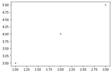
plt.plot(np.array([1,2,3]),np.array([3,4,5]),'.')
- 예제들
t=np.linspace(-6,6,100)
t
array([-6. , -5.87878788, -5.75757576, -5.63636364, -5.51515152,
-5.39393939, -5.27272727, -5.15151515, -5.03030303, -4.90909091,
-4.78787879, -4.66666667, -4.54545455, -4.42424242, -4.3030303 ,
-4.18181818, -4.06060606, -3.93939394, -3.81818182, -3.6969697 ,
-3.57575758, -3.45454545, -3.33333333, -3.21212121, -3.09090909,
-2.96969697, -2.84848485, -2.72727273, -2.60606061, -2.48484848,
-2.36363636, -2.24242424, -2.12121212, -2. , -1.87878788,
-1.75757576, -1.63636364, -1.51515152, -1.39393939, -1.27272727,
-1.15151515, -1.03030303, -0.90909091, -0.78787879, -0.66666667,
-0.54545455, -0.42424242, -0.3030303 , -0.18181818, -0.06060606,
0.06060606, 0.18181818, 0.3030303 , 0.42424242, 0.54545455,
0.66666667, 0.78787879, 0.90909091, 1.03030303, 1.15151515,
1.27272727, 1.39393939, 1.51515152, 1.63636364, 1.75757576,
1.87878788, 2. , 2.12121212, 2.24242424, 2.36363636,
2.48484848, 2.60606061, 2.72727273, 2.84848485, 2.96969697,
3.09090909, 3.21212121, 3.33333333, 3.45454545, 3.57575758,
3.6969697 , 3.81818182, 3.93939394, 4.06060606, 4.18181818,
4.3030303 , 4.42424242, 4.54545455, 4.66666667, 4.78787879,
4.90909091, 5.03030303, 5.15151515, 5.27272727, 5.39393939,
5.51515152, 5.63636364, 5.75757576, 5.87878788, 6. ])x=np.sin(t)
y=np.cos(t)plt.plot(t,x)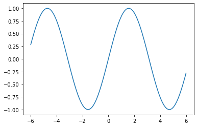
plt.plot(t,y)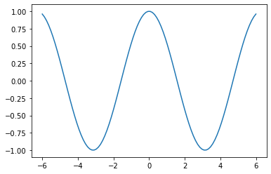
plt.plot(t,x)
plt.plot(t,y)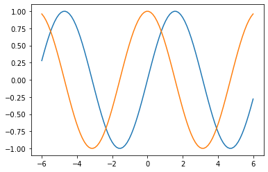
plt.plot(t,x)
plt.plot(t,y,'.')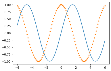
plt.plot(t,x)
plt.plot(t,y,'--')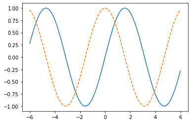
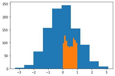
plt.hist
X=np.random.randn(1000)plt.hist(X)(array([ 3., 14., 66., 157., 232., 245., 155., 92., 28., 8.]),
array([-3.29472542, -2.65210581, -2.0094862 , -1.36686658, -0.72424697,
-0.08162736, 0.56099226, 1.20361187, 1.84623148, 2.4888511 ,
3.13147071]),
<BarContainer object of 10 artists>)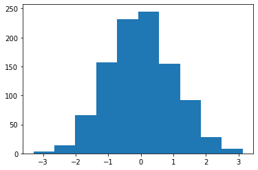
Y=np.random.rand(1000)
plt.hist(Y)
(array([ 98., 127., 107., 87., 83., 86., 85., 118., 110., 99.]),
array([0.00162071, 0.10140453, 0.20118836, 0.30097218, 0.40075601,
0.50053983, 0.60032366, 0.70010748, 0.79989131, 0.89967513,
0.99945896]),
<BarContainer object of 10 artists>)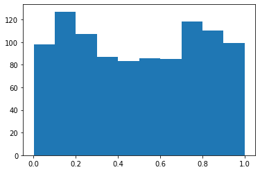
plt.hist(X)
plt.hist(Y)
(array([ 98., 127., 107., 87., 83., 86., 85., 118., 110., 99.]),
array([0.00162071, 0.10140453, 0.20118836, 0.30097218, 0.40075601,
0.50053983, 0.60032366, 0.70010748, 0.79989131, 0.89967513,
0.99945896]),
<BarContainer object of 10 artists>)